In the previous post we looked at the OLTP systems as the origin of state change data. Let’s take a look at the other side of the fence now.
When we were talking about collecting historical data from our OLTP system for analytics purposes we were sending this data “elsewhere” for further analysis. This place can have many names, shapes, and forms, but they all fit under the category of systems called OLAP (online analytical processing). While OLTP systems execute fundamental business tasks, OLAP system goals are to provide visibility into how such tasks are running, assist with planning, reporting, audit, and decision making.
Properties of such systems:
- Store large amounts of historical data (usually forever)
- Data from many OLTP systems is consolidated to provide a single business-wide view
- Have a much lower transaction rate than OLTP
- User queries are mostly read-only
- Queries can be very complex and involve a lot of aggregations
- Queries can be long-running, it’s common to see periodic batch processing and streaming workloads
- The set of queries frequently changes and they may be left up to the users to construct
Facts and Dimensions #︎
Let’s see how we could build a schema for analyzing transactions in our online game store:
| TransactionID | EventTime | AccountID | SkuID | Settlement |
|---|---|---|---|---|
| 1 | T1 |
1 | 3 | -100 |
| 2 | T2 |
5 | 4 | -400 |
| 3 | T3 |
9 | 0 | 500 |
This table can track every change to the players’ account balance, including store purchases and currency grants. This type of table is commonly known as a “fact” table - one that captures the high-frequency events that happen in your business.
Fact tables usually have one or more numerical values associated with them (Balance and Debit in our case). It is rare for a data analyst to look at the values of every fact individually, so these values are usually aggregated by some criteria. For example. we could aggregate how much money each player spent this month as:
|
|
In addition to facts, we also have “dimensions”. The OLAP dimensions allow us to associate some contextual information with each fact. Dimensions are identifiers that may reference other tables in our schema. For example SkuID adds context around which SKU was purchased by a player as part of the transaction.
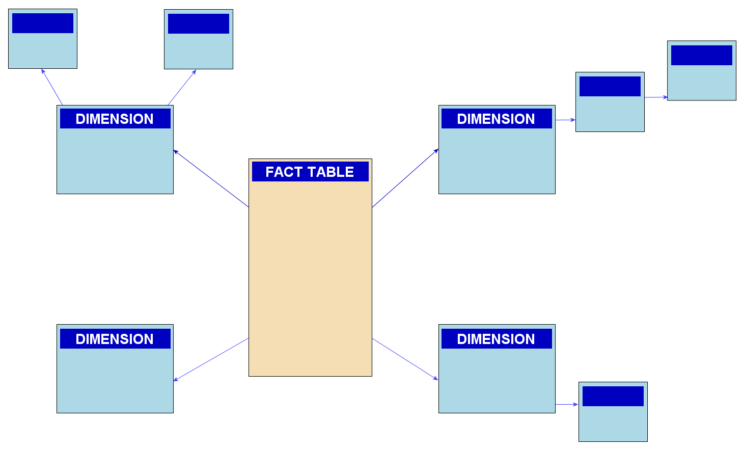
Snowflake Schema
The model with the fact table containing references to a bunch of dimensions is commonly known as a “star” or a “snowflake” schema. For allowing us to look at data from a bunch of different perspectives, projecting away some dimensions and aggregating the values, this model is also known as an “OLAP cube” or a “pivot table”.
Slowly Changing Dimensions #︎
In the fact table. we are explicit about the time dimension - every event has a timestamp associated with it. In OLAP most dimensions are not frozen in time either. Even though with a much slower frequency than adding new facts, dimensions change over time.
For example, if in our OLTP game store application SKUs were mutable, and the price of SKU can be changed by the content designer - we would need to somehow capture these changes in OLAP. If SKU price was changed from 100 to 50 during a promotion it would be incorrect for us to associate facts before and after promotion with the same SKU entity.
What do we do? We can say that before and after any changes these SKUs are actually different entities:
| SkuID | EffectiveFrom | EffectiveTo | Price |
|---|---|---|---|
| 1 | T1 |
T2 |
100 |
| 1 | T2 |
NULL | 50 |
The process of capturing such changes is known as “historization”, and the problem of modeling such changes in relational databases is known as “slowly changing dimensions” problem (SCD).
There are multiple SCD model types which are very simple and you can review them yourself. The example above is using SCD Type 2 with effective time ranges.
What we are essentially doing here is translating the mutable concept of an SKU from the OLTP system into an immutable one. Note that this is the case where making SKUs immutable by design in OLTP system would make the life of OLAP developers so much easier.
It is straightforward to navigate from any fact to the exact state of the SKU it is associated with. When querying SKUs not by primary key, however, special care should be taken to account for effective time ranges. Dealing with time ranges in queries, primary key and interval constraints, and in referential integrity can be quite tedious, so SQL:2011 standard adds special features for dealing with temporal data (a highly recommended read).
Different Kinds of Time #︎
We weren’t building GPS satellites or solving astrophysics problems, but if you paid attention you could see that we already introduced the “relativity” of time. There were two different kinds of time we were dealing with in our examples:
- System time
- Application time
Since our OLTP system is an authoritative source of online store data (that is the entities like SKU, account, balance, etc. originate in that system), all temporal information for its entities was recorded using “system time”. In the simplest form - whenever we made any modifications to data we could use CURRENT_TIMESTAMP SQL function to associate system time with it. This time is also known as “transaction time”.
The OLAP system also has its own system time, and if the clocks are perfectly in sync it would be the same as system time of the OLTP system. But the OLAP system stores the information about entities that are external to it. Depending on your architecture, it can take from milliseconds to several days for history from OLTP system to propagate to OLAP. No matter how small the window is - it’s non-zero. The EventTime, EffectiveFrom, and EffectiveTo times in our examples were, in fact, different kinds of time - SQL:2011 calls it “application time”, but it’s also known as “valid time”.
To prove to you that this is not just a different time but actually a different kind of time - there is no relationship between OLAP system’s system time (CURRENT_TIMESTAMP) and the application time (e.g. EventTime), and any comparisons between them are meaningless. Events will usually arrive late, so seeing T on a system time clock doesn’t exclude that facts with application time T-1 can appear later on. There are cases as we’ll see later when the opposite is true - application time can go arbitrarily far into the future compared to the system time.
Bitemporal Data #︎
So far we’ve only seen either one or another kind of time manifesting itself in our models. But there are cases when we would need both.
Leading with an example, imagine we want to implement a feature allowing a content designer to set up promotions to offer some SKUs at a discounted price. We don’t really want them to run SQL queries on the Christmas eve, so we need to be able to schedule promotions ahead of time. The application time we previously only used in OLAP now making its appearance in OLTP:
| SkuID | EffectiveFrom | EffectiveTo | Price |
|---|---|---|---|
| 1 | Ta1 |
Ta2 |
100 |
| 1 | Ta2 |
Ta3 |
50 |
| 1 | Ta3 |
NULL | 100 |
Remember I promised you an example where application time can be arbitrarily in future compared to system time? Well, here it is.
Now imagine that by some horrible mistake the promotion price was set to 5000 instead of 50. In the online game store it’s not that big of a deal - most people simply won’t buy the item, and if some will - good for us. But if we were dealing with real cash or we were a supplier of some manufacturing parts and our customers had this SKU on auto-purchase in their inventory management software - we would surely be held accountable.
If we discover the problem at the time between Ta2 and Ta3 when this broken “promotion” is in effect, what can we do? We could jump in and modify 5000 back to 50, but some purchases could already go through. We would also be erasing all the history of our mistake from the system.
Welcome to bitemporal data models!
The initial state of the system (mistake introduced):
| SkuID | SysFrom | SysTo | EfFrom | EfTo | Price |
|---|---|---|---|---|---|
| 1 | Ts1 | NULL | Ta1 | Ta2 | 100 |
| 1 | Ts2 |
NULL |
Ta2 | Ta3 | 5000 |
| 1 | Ts2 | NULL | Ta3 | NULL | 100 |
Correcting the mistake:
| SkuID | SysFrom | SysTo | EfFrom | EfTo | Price |
|---|---|---|---|---|---|
| 1 | Ts1 | NULL | Ta1 | Ta2 | 100 |
| 1 | Ts2 | Ts3 |
Ta2 | Ta3 | 5000 |
| 1 | Ts2 | NULL | a3 | NULL | 100 |
| 1 | Ts3 |
NULL |
Ta2 | Ta3 | 50 |
The way to interpret this is:
SysFromis effectively the time when any row was created in our database- The promotion was created at the time
CURRENT_TIMESTAMP == Ts2 SysTois the time when any row was deleted- Note that updates in this model expressed by deleting an old row and inserting an updated version of it as a new row
- We correct the error at time
CURRENT_TIMESTAMP == Ts3by “updating” the incorrect row (by settingSysTo = Ts3on old row and inserting correct one withSysFrom = Ts3as a single transaction) - The full history of what happened can be still reconstructed from data - all our changes were non-destructive
- An interesting property of such model is that all columns are immutable with the exception of
SysTo
One intuitive way of thinking about bitemporal data is:
- Application time intervals reflect the time during which a certain statement (proposition) that our table is capturing was/is/will be true to the best of our knowledge. Our knowledge can change, and as it does we update the propositions.
- System time captures the history of how our knowledge was changing over time. History once written is immutable.
- Application time is an interval when we believe a proposition P was/is/will be true
- System time is an interval when the proposition “proposition P is true” was true
…(sound of brain exploding)…
Remember the “AS OF” proejction from SQL:2011? We used it to move back to any point in time. With bitemporal model, there are now two kinds of projections (I’m switching to a somewhat colloquial terminology here which unfortunately does not align well with AS OF meaning from SQL:2011):
AS ATor “As we knew at that time”. This projection collapses the system time dimension. If we would go to a time right beforeTs3- this is the time when the error in the database was not corrected yet. This projection shows us what really happened.AS OFor “As we should have known”. This projection collapses the application time dimension. If we would now go to a timeTa2we would see the SKU price of50, with the correction applied. This projection tells us what should’ve happened.
By diffing the results of two projections we can understand which purchases were affected by the error and which customers should be compensated. We preserve a complete record of everything that ever happened!
Let this idea soak in for a bit…
If this doesn’t impress you - I don’t know what will!
Time in Stream Processing Systems #︎
Research on (bi)temporal systems has been active for the last 25-30 years, but it only found its use in a handful of specialized software. Interestingly enough the most prominent example of bitemporal data making its way into the “mainstream” software architecture nowadays is the stream processing systems.
The time when an event is emitted and the time when it is processed by the system can greatly vary. When your event source is on a mobile network events can be late by minutes or even days, can arrive late and in random order. So weather you know it or not - stream processing is a bitemporal system.
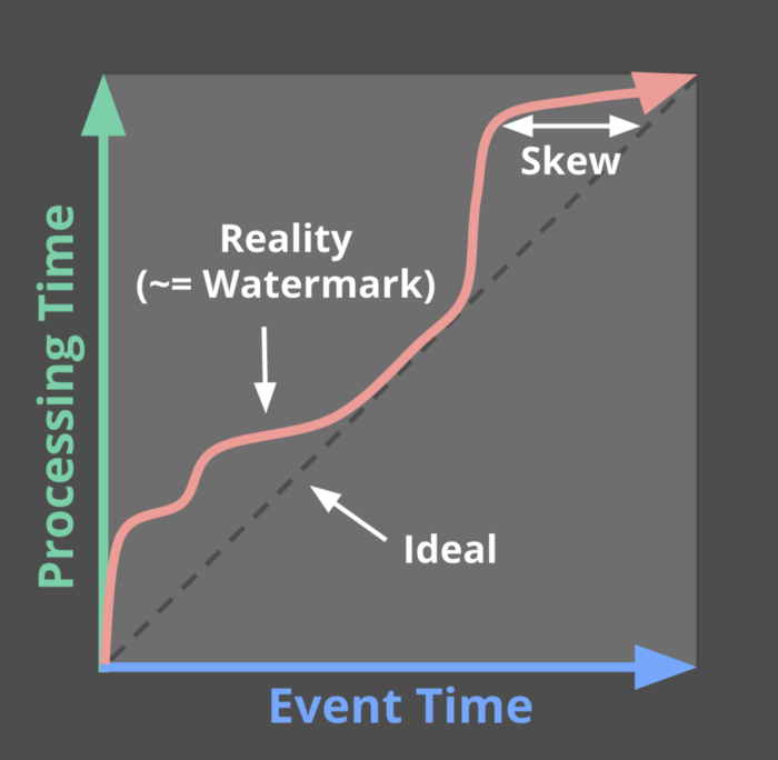
Modern stream processing tools rely on sophisticated windowing techniques, heuristic watermarking, and triggers to reconcile the differences between these two kinds of time. This topic requires a detailed explanation and already well covered, so I will refer you to these articles:
Time Dimension in the World of Hadoop and Spark #︎
The birds-eye view of the processing chain we had so far is:
- OLTP system implements business rules and controls state transitions
- State transitions are captured via one of the methods we described earlier and exposed
- Data in transit, as we called it, is then ingested into an OLAP system
- Data is transformed, structured, historized
- Data is made available for efficient querying in form of OLAP cubes
This is a classic ETL (extract-transform-load) process, at the end of which you get a “data mart” database with a clean (temporal) relational model.
Nowadays OLAP systems are moving towards ELT (extract-load-transform) process. The idea behind ELT is that the ingestion process finishes much earlier, right after raw data is written durably to some kind of a distributed storage (HDFS, S3). There is no heavy-weight transformation or other processes after that. Later this data is consumed by potentially multiple different analytic systems with all necessary transformations are performed as part of querying the data.
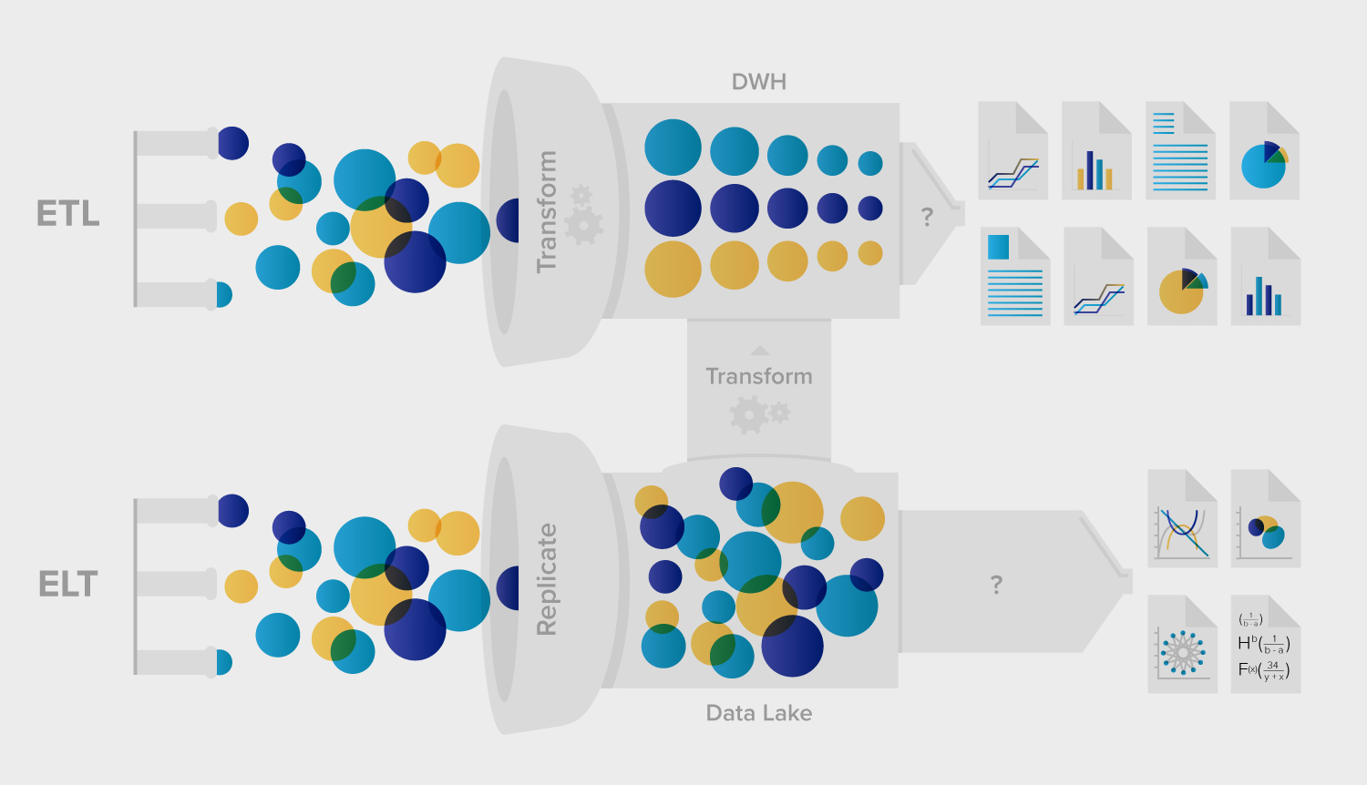
You might’ve heard expression “schema-on-read” - in this philosophy each query reads only the minimal subset of data it needs and ignores the rest - this is much more flexible than waiting for data team to update their OLAP cubes to recent changes in applications. Query performance is achieved via massive parallelism using distributed processing engines such as Spark. The selective nature of queries that read only data that matters to them is taken into account in modern structured columnar storage formats like Parquet and ORC. You can think of these formats as a relational-table-in-a-file. Unlike a DB table however, these formats are immutable, which suits our use case nicely because domain events once emitted cannot be changed.
The fact that queries operate on raw events doesn’t mean that (bi)temporal relational data models are not relevant any more. Data in event form is optimal for a needle-in-a-haystack queries and stream-to-stream joins, while (bi)temporal relational representation is helpful when you need fast projections, set operations, and temporal joins. So depending on a query, building temporal models may simply be one of the pre-processing steps. We scan the events, aggregate them into temporal tables, then run our queries, joins, etc. If temporal queries are frequent it’s within ELT best practices to employ stream processing to maintain an up-to-date temporal “view” of the event data.
Does this change how we represent the data in transit?
Only a little. Previously we were saying that it doesn’t matter how you serialize the domain events because ETL process would deal with them one by one. Now in the interest of performance, it is best to store events in a structured format suitable for parallel processing (see aforementioned Parquet and ORC).
Conclusion #︎
In the modern digital world data is our history, and it pains me to see how negligent we currently are in preserving it. Increase in storage requirements for a while now has not been a valid excuse, we have all the means to preserve our digital history. The learning curve of maintaining and most importantly utilizing the benefits of temporal data remains steep. The tooling is significanlty lacking in this respect and needs to step up for us to propell the cost-benefit loop.
In these two posts we narrowed down on what’s the most optimal way to capture data changes is, and how these changes should be exposed for further processing, but it’s not realistic that all data sources will adapt any time soon. In Kamu we are utilizing the techniques we covered here to transform snapshot data published on the web into the historical form at the moment of ingestion. So even though data sources themselves don’t provide us with change history we can capture it by periodically observing the snapshots and reconstructing how they evolved.